Ionisation potential of a porous material#

In this example we use MacroDensity with VASP to align the energy levels of a porous material.

The procedure involves one DFT calculaion, yielding different important values:

\(\epsilon_{vbm}\) - the valence band maximum
\(V_{vac}\) - the vacuum potential

The ionisation potential (\(IP\)) is then obtained from:

\(IP = V_{vac} - \epsilon_{vbm}\)

The difference to a bulk calculation is that here the material itself has a vacuum within it. This allows us to sample the vacuum level from the vacuum region, as explained in this paper.

Our system#

We will demonstrate this procedure for the porous system ZIF-8.

Procedure#

Optimise the structure
Calculate the electronic structure at your chosen level of theory, adding the LVHAR flag to the INCAR file:

LVHAR = .TRUE. # This generates a LOCPOT file with the potential
Locate the centre of the largest pore - do this “by eye” first
Plot the potential in that plane, so see if it plateaus
Plot a profile of the potential across the pore, again to see the plateau
Sample the potential from the pore centre

Look for pore centre points#

For this we will use VESTA.
- Open the LOCPOT in VESTA.
- Expand to 2x2x2 cell, by choosing the Boundary option on the left hand side.
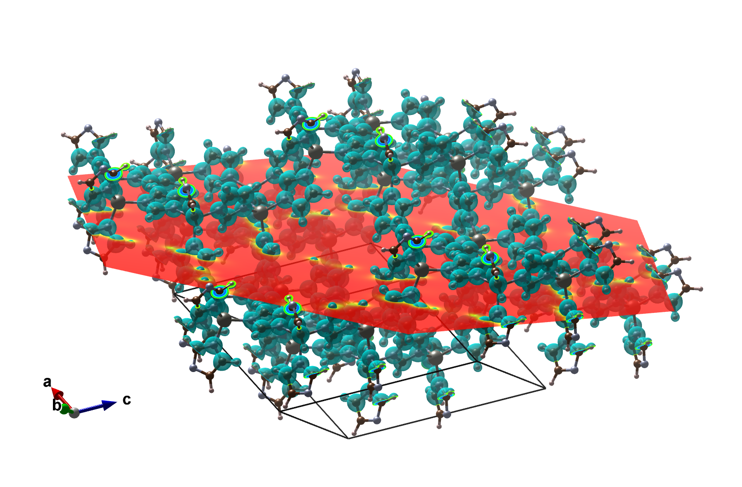
- Look for a pore centre - [1,1,1] is at a pore centre here.
- Now draw a lattice plane through that point.
  - Choose Edit > Lattice Planes.
  - Click New.
  - Put in the Miller index (e.g. 1,1,1).
  - Move the plane up and down using the d parameter, until it passes through the point you think is the centre.
  - It should look like the picture below.
Now we look at a contour plot of this plane to see if we are at a plateau.
- Utiltiy > 2D Data Display.
- Click Slice and enter the same parameters as in the 3D view.
- Now choose contours to play with the settings
- Z(max) and Z(min) tell you the potential max and min.
- Set contour max = Z(max) and contour min = 0 and the interval to 0.1.
- With some playing with the General settings, you can get something like this:

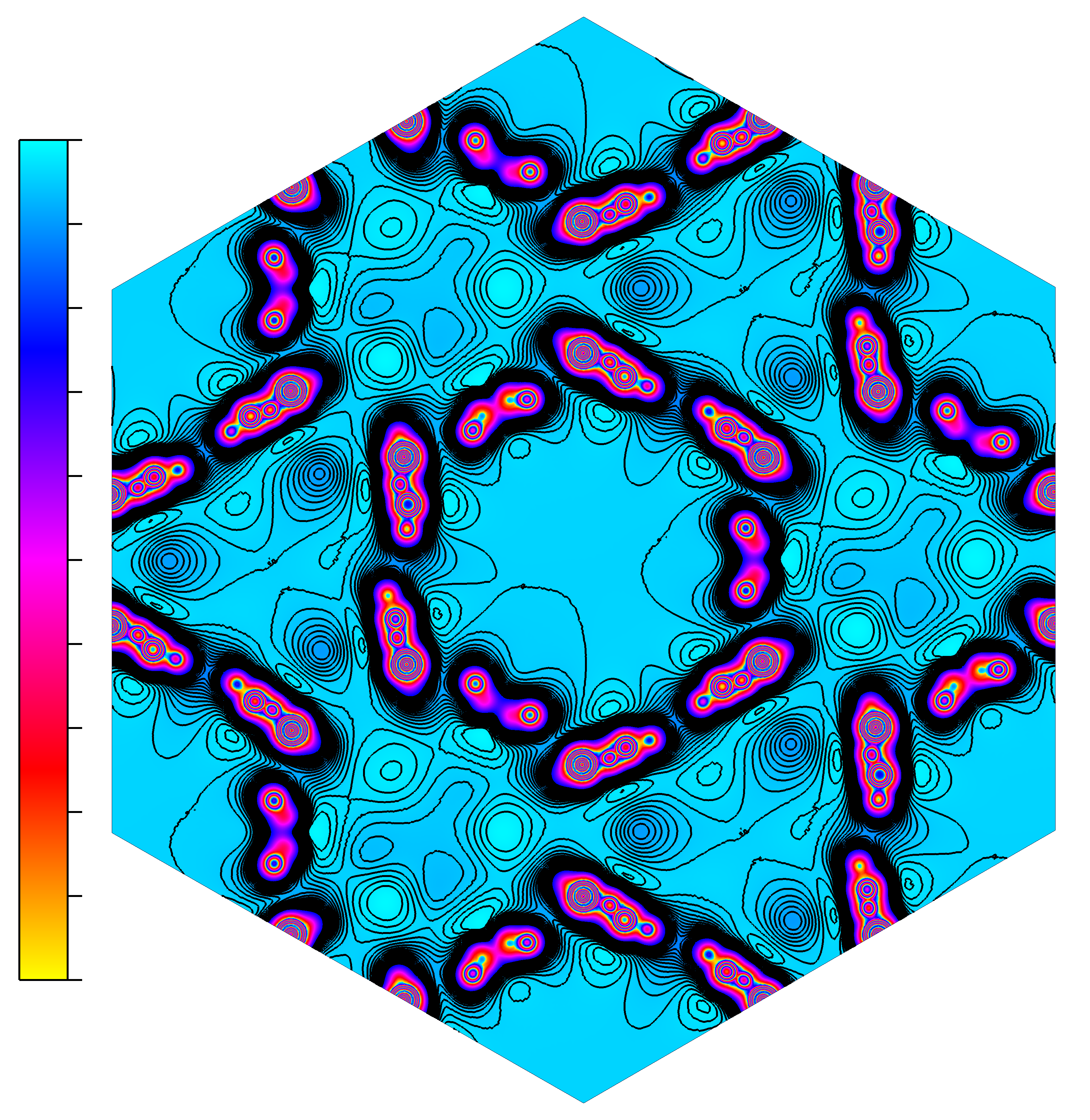
We can see the [1,1,1], at the centre of the picture is a maximum and is a plateau, so we can now use it for sampling.

Sampling the potential#

We now set the point to sample at [1,1,1]
We must also set the travelled parameter, for this type of analysis it is always [0,0,0].

Read the potential#

%matplotlib inline
%load_ext autoreload
%autoreload 2

import sys
sys.path.append('../../')
import imp
import macrodensity as md
import math
import numpy as np
import matplotlib.pyplot as plt
import os

The autoreload extension is already loaded. To reload it, use:
  %reload_ext autoreload

if os.path.isfile('LOCPOT'):
    print('LOCPOT already exists')
else:
    os.system('bunzip2 LOCPOT.bz2')

LOCPOT already exists

# Read the potential from the LOCPOT file
input_file = 'LOCPOT'

vasp_pot, NGX, NGY, NGZ, Lattice = md.read_vasp_density(input_file)
vector_a, vector_b, vector_c, av, bv, cv = md.matrix_2_abc(Lattice)
grid_pot, electrons = md.density_2_grid(vasp_pot, NGX, NGY, NGZ)

Reading header information...
Reading 3D data using Pandas...
Average of the potential =  1.9559870102655787e-14

cube_origin = [1,1,1]
travelled = [0,0,0]

We want to try a range of sampling area sizes and analyse how this affects the potential.
We also want low variance (plateau condidtions).
Ideally we should have as large an area as possible, with low (< 1e-5) variance.

dim = [1, 10, 20, 40, 60, 80, 100]
print("Dimension   Potential   Variance")
print("--------------------------------")
for d in dim:
    cube = [d, d, d]
    cube_potential, cube_var = md.volume_average(
        cube_origin, cube, grid_pot, NGX, NGY, NGZ, travelled=travelled
    )
    print(f"{d}\t    {cube_potential:.4f}\t   {cube_var:.5f}")

Dimension   Potential   Variance
--------------------------------
   2.3068	   0.00000
   2.3068	   0.00000
   2.3068	   0.00000
   2.3068	   0.00002
   2.3067	   0.00011
   2.3048	   0.00115
   2.2883	   0.01587

So we take the potential value of 2.3068. For the VBM value, we take it from the OUTCAR file (VBM: -2.4396 eV)

vbm = -2.4396 # eV
print("IP: %3.4f eV" % (2.3068 - vbm))

IP: 4.7464 eV

Ionisation potential of a porous material

Contents